From Statistics To Lack Of Fit Test

According to Alan Turing, a system, which probably looks pretty complicate, can be described with simple mathmatical equation. In machine learning domain, the models can be usually interpreted with equations, and the parameters of "equations" is what we want to learn. Usually, the parameter we finally get is an estimator of the real value. But how do we describe how good the estimator is?

Let's start with the Estimator.

The parameter is a quantity of a real model e.g. the mean or the variance of random variable, the parameter of a probability distribution, etc. An estimator, according to Wikipedia is a rule for calculating an estimate of parameter based on observed data. Because the estimator is calculated by a function of observed data, so the estimator is itself also random variable. (This concept is also the main idea of Bayesian Model in machine learning).

Suppose we want to know a paramter \(\theta\), which can be estimated by a sample set \(D_{S}\) drawn from \(X\). \(\hat{\theta}_S(X)\) is denoted as the estimator of \(\theta\) based on observed data of random variable \(X\). Let's denote \(x\) as a particular obseved data \(X=x\). Sampling is an approximation of the real world. So it could happen that for some reasons the sample set doesn't represent the real issuse very well. There are some important quantified properties which are helpful before we dive deeper.

What hint can we get from bias and variance of estimator when doing model fitting? Suppose we have a model \(f(x)\) in the real world, due to the noise we get caught into the delimma that we never observe the real \(f(x)\) given an \(x\), but the noisy data \(y=f(x)+\epsilon\). Following the workflow of regression we should first of all find a function family to fit the model. suppose we come up with polynomial \(p_N(x)=a_0+a_1x+ a_2x^2+...+a_Nx^N\). Training, testing… How good performance will we finally get?

To find out the real model precisely is difficult, two main probelems exist as the following figure shows.

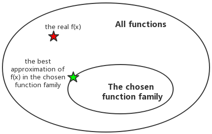
• Suppose \(f(x)\) is the real model. The function family we choose, e.g. like the polynomial family, may not include the \(f(x)\). This may be caused by lack of domain knowledge or so on.
• We may not even get the best approaximation \(\hat{f}_{best}(x)\) out of the chosen functioon family. This can blame on not good enough sampling, overfitting, underfitting and so on.

How do we assess the prediction performance? So suppose we finally choose \(p(x)\) as the prediction function. Noted that the prediction function is based on the data, so the prediction function is random variable. If we repeatedly and independently sample data several times, we get different \(g(x)\). The expected value of \(p(x)\) is \(E[p(x)]\). There are some parameters to be introduced:

• The variance can be denoted as \(Var = E[(p(x)-E[p(x)])^2]\).
• The bias is \(Bias = E[p(x)] - f(x)\).
• The prediction error is \(E[(p(x)-y)^2]\), i.e. the mean square of error btw. the predicted value and observed value.
• The expected value of \(y\) supposed to be \(f(x)\) if the noise is with zero expected value. (E.g.zero-mean Gaussian noise)
• If the noise is unbiased, \(\sigma^2\) quantifies how much the responses \(y\) vary around the (unknown) mean regression line(the real model) \(f(x)\).

Fed with these concepts, we can actually compare them with the former chapter on estimator bias and variance and MSE. Try to replace θ with y, \(\hat{\theta}\) with \(p(x)\), and \(E[\hat{\theta}]\) with \(E[p(x)]\), then you can find the relationship.

Let's explore the underlying relationship. A given observed \((x^*,y^*)\) pair is drawn due to \(y^*=f(x^*) + \epsilon\). For a given set of pbserved data pairs, the expected prediction error is \(E[(p(x^*)-y^*)^2]\). We expand it as:

\begin{align*} E[(p(x^*)-y^*)^2] &= E[p^2(x^*)] - 2E[p(x^*)y^*] + E[{y^*}^2] \\ &= E[p^2(x^*)] - 2E[p(x^*)]f(x^*) + E[{y^*}^2] \end{align*}

Since:

\begin{align*} E[p^2(x^*)] &= E[(p(x^*) - E[(p(x^*)])^2] +E^2[p(x^*)] \\ E[{y^*}^2] &= E[(y*-E[y^*])^2] +E^2[y^*] = E[(y*-f(x^*))^2] +f^2(x^*) \end{align*}

So finally we can form the expected prediction error as:

\begin{align*} E[(p(x^*)-y^*)^2] &= E[(p(x^*) - E[(p(x^*)])^2] +E^2[p(x^*] - 2E[p(x^*)]f(x^*) + E[(y^*-f(x^*))^2] +f^2(x^*)\\ &= E[(p(x^*) - E[(p(x^*)])^2] + E[(y^*-f(x^*))^2] + E^2[p(x^*] -2E[p(x^*)]f(x^*)+f^2(x^*)\\ &= E[(p(x^*) - E[(p(x^*)])^2] + E[(y^*-f(x^*))^2] + (E[p(x^*)]-f(x^*))^2 \end{align*}

Notice that whatever effort we make, we can't eliminate the noise term of the error.

You may heard of the term "lack-of-fit sum of squares". There exists a relationship that the residual sum of squares can be decomposed into two components: lack-of-fit sum of squares and sum of squares of the differences between each observed $y$-value and the average of all y-values corresponding to the same $x$-value.

If you compare it carefully with the relationship mentioned above, you can find that the lack-of-fit dependens on the bias estimator and the noise. As said before, the noise is our delimma, however we do can improve our learning algorithm to minimize the bias estimator. Also I quote some figures to intuitively explain the variance estimator and bias estimator.

The following figures are cited from Model Selection: Underfitting, Overfitting, and the Bias-Variance Tradeoff

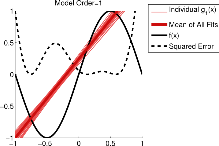
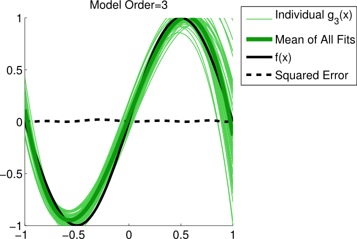
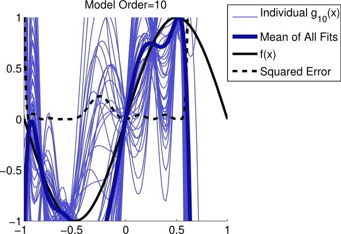
The real model is \(f(x)=sin(\pi x)\) The real world with noise is \(y= f(x)+ N(0,\sigma^2)\) Using the polynomials with \(N=1\), \(N=3\), and \(N=10\) seperately fit the observed data. The data are independently sampled 50 times and for each \(N\) there are 50 prediction functions. The first figure shows us that the model can't capture the real features of the data. It is sensible neither to the real model nor to the noise. So we can see that the variance of those 50 lines is low. But the bias is high. So this is a typical case of underfitting. The third figure in the contrast, capture the real features and and also the noise we don't want. It is sensible not only to the real model but also to the noise. This time, however, we can see that the variance of those 50 lines is low. That's because it regards the noise as a feature, this is a typical case of overfitting. The best is the second figure. As we can see, it has relative lower bias and lower variance. The noise doesn't misguide our model.

So the trade-off is actually very parently. If we use a complex model with too much parameters, the model works well on the training data to lower the residules down. However, it may work very bad on test data, cause the model we get represents not only the real model but also the noise. It's not generalized. The bias may be very low but the variance goes too high. If the model is too simple, with not enough parameters, it probably doesn't capture the real features of the real model. So the bias may be very high in spite of lower variance.

the reference Test if the feature is correlated to the respond y There are two alternative methods for testing whether a linear association exists between the predictor x and the response y in a simple linear regression model, y=b₀+b_1x +ε

\begin{equation} H_0: b_1=0 vs. H_1: b_1 \neq 0 \end{equation}

• t-test for the slope
• analysis of variance (ANOVA) F-test

Firstly, specify the null \(H_0\) and alternative hypotheses \(H_1\) or \(H_A\).

Secondly, calculate the value of the test statistic according to the methode you use.

At last, use the resulting test statistic to calculate the P-value.

The p-value is a measure of the strength of the evidence and even extremer eveidence against the null hypothesis. It means that, if \(H_0\) is true, how likely will the observed value and even greater value appear.

By the way, the test statistic could be t-statistic, representing t-test, and F-statistic, representing F-test. These two methode are common used.

Once again, I list these concepts together.

1. Online-Course of Eberly College of Science
2. Model Selection: Underfitting, Overfitting, and the Bias-Variance Tradeoff
3. MSE and Bias-Variance decomposition
4. Deep Learning (Adaptive Computation and Machine Learning series)